[파이썬 라이브러리를 활용한 머신러닝] 지도학습(2)

파이썬 라이브러리를 활용한 머신러닝 책 내용 정리 포스트

Posted Sep 13, 2022 Updated Sep 14, 2022

By Seojin Park

25 min read

2.3 지도 학습 알고리즘

2.3.3 선형 모델

선형 모델이란?

입력 특성에 대한 선형 함수를 만들어 예측을 수행

회귀의 선형 모델

\[\hat{y} = w[0] * x[0] + w[1] * x[1] + \cdots + w[p] * x[p] + b\]

$x[0],x[1], \cdots ,x[p]$ : 데이터 포인트에 대한 특성(특성의 개수 : p + 1)
$w, b$ : 파라미터
$\hat{y}$ : 모델이 만들어낸 예측값

ex) feature = 1 → $\hat{y} = w[0] * x[0] + b$

feature ↑ → w는 각 feature에 해당하는 기울기를 모두 가짐

예측값 = (입력 특성) $\times$ (w의 각 가중치 : 음수도 가능) 의 합

  
mglearn.plots.plot_linear_regression_wave()

# w[0]: 0.393906  b: -0.031804

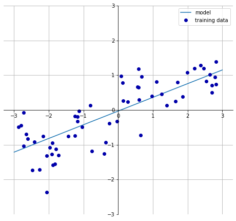
선형 회귀는 특성이 많은 데이터셋이거나 훈련 데이터보다 특성이 더 많은 경우에 유용하다.

선형 회귀(최소제곱법)

가장 간단하고 오래된 회귀용 선형 알고리즘
예측과 훈련 세트에 있는 타깃 y사이의 평균제곱오차를 최소화하는 파라미터 w와 b를 찾는 방식

평균제곱오차: 예측값과 타깃 값의 차이를 제곱하여 더한 후에 샘플의 개수로 나눈 것

선형 회귀의 장점은 매개변수가 없는 것이고 단점은 모델의 복잡도 제어할 방법이 없다.

  
from sklearn.linear_model import LinearRegression
X, y = mglearn.datasets.make_wave(n_samples=60)
X_train, X_test, y_train, y_test = train_test_split(X,y, random_state=42)

lr = LinearRegression().fit(X_train, y_train)

# 기울기 파라미터(w) : 가중치(weight) or 계수(coefficient) --> lr 객체의 coef_ 속성에 저장 (NumPy array)
# 파라미터(b) : 편향(offset) or 절편(intercept) --> intercept_ 속성에 저장 (float)

print("lr.coef_:", lr.coef_)
print("lf.intercept_:", lr.intercept_)

"""
lr.coef_: [0.39390555]
lf.intercept_: -0.031804343026759746
"""

print("Training set score: {:.2f}".format(lr.score(X_train, y_train)))
print("Test set score: {:.2f}".format(lr.score(X_test, y_test)))

"""
Training set score: 0.67
    Test set score: 0.66
"""

Train set score과 Test set score 비슷한 경우에는 과소적합인 상태이다.

$R^2$ 값이 크지 않음
훈련 세트와 테스트 세트의 점수가 매우 비슷

특성이 작은 경우는모델이 단순하므로 과대적합이 될 가능성이 적지만 고차원 데이터셋(특성이 많은 경우)인 경우는 선형 모델의 성능이 매우 높아져 과대적합될 가능성이 높다.

  
# sample : 506개, feature : 104개
X, y = mglearn.datasets.load_extended_boston()

X_train, X_test, y_train, y_test = train_test_split(X, y, random_state = 0)
lr = LinearRegression().fit(X_train, y_train)

print("Training set score: {:.2f}".format(lr.score(X_train, y_train)))
print("Test set score: {:.2f}".format(lr.score(X_test, y_test)))

"""
Training set score: 0.95
Test set score: 0.61
"""

훈련 세트에서는 예측이 정확하지만 테스트 세트에서는 $R^2$ 값이 매우 낮다면 모델이 과대적합되었다고 해석할 수 있다. 이때는, 복잡도를 제어할 수 있는 리지 회귀 모델을 사용해야한다.

리지 회귀

회귀를 이용한 선형 모델이므로 예측 함수를 사용
가중치(w)선택 = 훈련 데이터를 잘 예측(최소적합법과 동일) + 추가 제약 조건을 만족

Goal
가중치(w)의 절댓값을 가능한 한 작게 만드는 것, 즉 w의 모든 원소가 0에 가깝게 되는 것 = 모든 특성이 출력에 주는 영향을 최소한으로 만듦.(기울기를 작게 함.)

규제(regularization) : 과대적합이 되지 않도록 모델을 강제로 제한하는 것을 의미 리지 회귀에서 사용하는 규제 방식 : L2 규제

  
from sklearn.linear_model import Ridge

ridge = Ridge().fit(X_train, y_train)
print("Training set score: {:.2f}".format(ridge.score(X_train, y_train)))
print("Test set score: {:.2f}".format(ridge.score(X_test, y_test)))
"""
Training set score: 0.89
Test set score: 0.75
"""

Conclusion

Training set 점수 : 선형 회귀 > 리지 회귀
Test set 점수 : 선형회귀 < 리지 회귀

선형 회귀(LinearRegression): 과대적합(overfitting)
리지 회귀(RidgeRegression) : 과대적합이 적어짐(덜 자유로운 모델이기 때문)

모델의 복잡도 → 훈련 세트 점수가 낮으므로 더 일반화된 모델이라고 할 수 있다.

Test set score 에 대한 성능이 중요하기 때문에 Ridge Model 을 선택

Ridge 모델의 특징

모델을 단순화 & 훈련 세트에 대한 성능 사이르 절충할 수 있는 방법을 제공
alpha 매개변수로 훈련 세트의 성능 대비 모델의 단순화 정도를 지정할 수 있음.

alpha ↑ → 계수가 0에 가까워짐

훈련 세트의 성능은 나빠짐
모델의 일반화에는 도움이 됨

  
# alpha 값이 큰 경우
ridge10 = Ridge(alpha = 10).fit(X_train, y_train)
print("Training set score: {:.2f}".format(ridge10.score(X_train, y_train)))
print("Test set score: {:.2f}".format(ridge10.score(X_test, y_test)))

"""
Training set score: 0.79
Test set score: 0.64
"""

# alpha 값이 작은 경우 --> test set score이 상승(성능이 상승)
ridge01 = Ridge(alpha = 0.1).fit(X_train, y_train)
print("Training set score: {:.2f}".format(ridge01.score(X_train, y_train)))
print("Test set score: {:.2f}".format(ridge01.score(X_test,y_test)))

"""
Training set score: 0.93
Test set score: 0.77
"""

alpha 값에 따른 coef_(기울기) 속성의 변화한다.

alpha 값이 크면 더 많은 제약이 있는 모델
coef_의 절댓값 크기가 작을 것

  
plt.plot(ridge10.coef_, '^', label = "Ridge alpha = 10")
plt.plot(ridge.coef_, 's', label = "Ridge alpha = 1")
plt.plot(ridge01.coef_, 'v', label = "Ridge alpha = 0.1")

plt.plot(lr.coef_, 'o', label = "LinearRegression")
plt.xlabel("list of coefficient")
plt.ylabel("coefficient size")
xlims = plt.xlim()
plt.hlines(0, xlims[0], xlims[1])
plt.xlim(xlims)
plt.ylim(-25,25)
plt.legend()
plt.show()

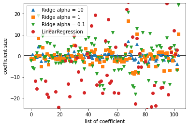
위의 그래프는 다음과 같다.

x = 0 인 경우 : 첫 번째 특성에 연관된 계수
x = 1 인 경우 : 두 번째 특성에 연관된 계수
y 축: 각 계수의 수치

alpha 값에 따른 계수의 크기

alpha = 10 → -3 ~ 3
alpha = 1 → alpha = 10일 때의 계수의 크기보다 큼
alpha = 0.1 → alpha = 1일 때의 계수의 크기보다 큼
규제가 없는 LinearRegression(alpha = 0) : alpha > 0 일 때 보다 큼

규제의 효과

alpha 값에 따른 계수의 크기를 비교하는 방법
alpha 값을 고정하고 훈련 데이터의 크기를 변화시키는 방법

  
# 규제의 효과 2번 방법
mglearn.plots.plot_ridge_n_samples()

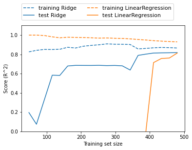
그래프 분석

목록	선형 회귀	리지
점수 비교	훈련 세트 점수 > 테스트 세트 점수	훈련 세트 점수 > 테스트 세트 점수
데이테 개수 400미만	학습이 이루어지지 않음	학습이 이루어지고 있음
데이터 개수 400이상	학습이 이루어짐	학습이 이루어짐
규제 유무	규제 없음	규제 있음
규제에 따른 훈련 세트 점수 비교	항상 더 큼	항상 더 작음

데이터의 개수가 많아질수록 성능은 좋아짐
데이터의 양이 많아지면 규제 항의 중요성이 낮아져 리지 회귀와 선형 회귀의 성능이 같아질 것
선형 회귀의 훈련 데이터 성능이 낮아짐 → 데이터의 양이 많아지면 모델이 데이터를 기억하기 어려움 & 과대적합하기 어려움

라소(Lasso)

Ridge의 대안으로 선형 회귀에 규제를 적용하는데 이용
계수를 0에 가깝게 만들려고 함 → L1 규제
실제로 어떤 계수는 0이 됨 → 완전히 제외되는 특성이 생김 = 특성 선택(feature selection)이 자동으로 이루어짐

즉, 일부 계수가 0으로 만들어지기 때문에 모델을 이해하기 쉬워지며 모델의 가장 중요한 특성이 무엇인지 분명하게 알 수 있음.

  
from sklearn.linear_model import Lasso

lasso = Lasso().fit(X_train, y_train)
print("Training set score: {:.2f}".format(lasso.score(X_train, y_train)))
print("Test set score: {:.2f}".format(lasso.score(X_test, y_test)))
print("Number of features used:",np.sum(lasso.coef_!=0))

"""
Training set score: 0.29
Test set score: 0.21
Number of features used: 4
"""

과소적합 → alpha 값을 증가
- 단, max_iter (= 반복 실행하는 최대 횟수)를 늘려야함
4개의 특성만 사용
alpha 매개변수 지원( 기본값 = 1.0)

  
# max_iter 기본값을 증가시키지 않으면 max_iter 값을 늘리라는 경고가 발생
lasso001 = Lasso(alpha = 0.01, max_iter = 50000).fit(X_train, y_train)
print("Training set score: {:.2f}".format(lasso001.score(X_train, y_train)))
print("Test set score: {:.2f}".format(lasso001.score(X_test,y_test)))
print("Number of features used:", np.sum(lasso001.coef_!=0))

"""
Training set score: 0.90
Test set score: 0.77
Number of features used: 33
"""

alpha 값 ↓ → 훈련 세트 & 테스트 세트 성능 ↑
사용된 특성 개수 : 33개 → 분석하기가 쉬움
Ridge 성능보다 좋음

  
# 과대적합된 경우(alpha 값이 너무 작음)
lasso00001 = Lasso(alpha = 0.0001, max_iter = 50000).fit(X_train, y_train)
print("Training set score: {:.2f}".format(lasso001.score(X_train, y_train)))
print("Test set score: {:.2f}".format(lasso001.score(X_test,y_test)))
print("Number of features used:", np.sum(lasso001.coef_!=0))

"""
Training set score: 0.90
Test set score: 0.77
Number of features used: 33
"""

plt.plot(lasso.coef_, 's',label = "Lasso alpha = 1")
plt.plot(lasso001.coef_, '^', label = "Lasso alpha = 0.01")
plt.plot(lasso00001.coef_, 'v', label = "Lasso alpha = 0.0001")

plt.plot(ridge01.coef_, 'o', label = "Ridge alpha = 0.1")
plt.legend(ncol = 2, loc = (0,1.05))
plt.ylim(-25,25)
plt.xlabel("list of coefficients")
plt.ylabel("coefficient size")
plt.show()

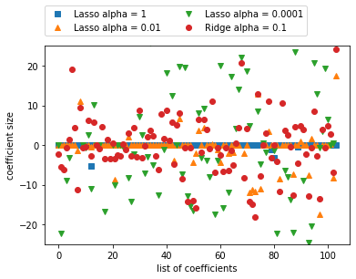
그래프를 분석하면 다음과 같이 분석할 수 있다.

alpha = 1 : 계수 대부분이 0 + 나머지 계수들도 크기가 작음
alpha = 0.01 : 대부분의 특성이 0
alpha = 0.0001 : 계수의 대부분이 0이 아니며 값이 큼(규제가 크지 않는 모델)
Ridge 모델과 alpha = 0.01인 모델과 비슷하지만 어떠한 계수도 0이 되지는 않음.

리지 vs 라소
리지 회귀를 선호함
특성이 많고 그 중 일부분만 중요한 경우에는 라소(Lasso)가 더 좋은 선택일 수 있음
분석하기 쉬운 모델을 선호 → Lasso
ElasticNet = Lasso + Ridge의 페널티
최상의 성능을 내지만 L1 규제와 L2 규제를 위한 매개변수 두 개를 조정해야함

  
from sklearn.linear_model import QuantileRegressor

X, y = mglearn.datasets.make_wave(n_samples = 60)
X_train, X_test, y_train, y_test = train_test_split(X, y, random_state = 42)

pred_up = QuantileRegressor(quantile = 0.9, alpha = 0.01).fit(X_train, y_train).predict(X_test)
pred_med = QuantileRegressor(quantile = 0.5, alpha = 0.01).fit(X_train, y_train).predict(X_test)
pred_low = QuantileRegressor(quantile= 0.1, alpha = 0.01).fit(X_train, y_train).predict(X_test)

plt.scatter(X_train, y_train, label = 'Training data')
plt.scatter(X_test, y_test, label = 'Test data')
plt.plot(X_test, pred_up, label = 'Quantile:0.9')
plt.plot(X_test, pred_med, label = 'Quantile:0.5')
plt.plot(X_test, pred_low, label = 'Quantile:0.1')
plt.show()

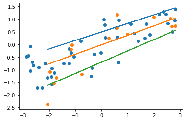
그래프를 분석하면 다음과 같이 분석할 수 있다.

백분위 이용
라소 모델과 비슷하게 alpha 매개변수로 L1 규제를 조정
alpha 매개변수 기본값 = 1.0
alpha 값 ↑ → 규제가 강해져 과소적합한 모델을 만듦

분류용 선형 모델

이진 분류인 경우

$\hat{y} = w[0] * x[0] + w[1] * x[1] + … + w[p] * x[p] + b > 0$

0과 비교	클래스
예측값 > 0	+1
예측값 < 0	-1

case 1. 회귀용 선형 모델

출력 ŷ이 특성의 선형 함수(직선, 평면, 초평면)

case 2. 분류용 선형 모델

결정 경계가 입력의 선형 함수 = (이진) 선형 분류기는 선, 평면, 초평면을 사용해 두개의 클래스를 구분하는 분류기

선형 모델 학습 알고리즘

특정 계수와 절편의 조합이 훈련 데이터에 얼마나 잘 맞는지 측정하는 방법
사용할 수 있는 규제가 있는지, 있다면 어떤 방식인지

단, 잘못된 분류의 수를 줄이기 위해 w와 b를 조정하는 것은 불가능

선형 분류 알고리즘

로지스틱 회귀(logistic regression)
서포트 벡터 머신(support vector machine)

  
from sklearn.linear_model import LogisticRegression
from sklearn.svm import LinearSVC

X, y = mglearn.datasets.make_forge()

fig, axes = plt.subplots(1, 2, figsize = (10, 3))

for model, ax in zip([LinearSVC(max_iter = 5000), LogisticRegression()], axes):
  clf = model.fit(X, y)
  mglearn.plots.plot_2d_separator(clf, X, fill = False, eps = 0.5,ax = ax, alpha = .7)
  mglearn.discrete_scatter(X[:,0], X[:,1], y, ax = ax)
  ax.set_title(clf.__class__.__name__)
  ax.set_xlabel("feature 0")
  ax.set_ylabel("feature 1")
axes[0].legend()
plt.show()

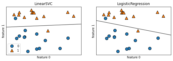
LinearSVC & Logistic Regression 모두 L2 규제(제곱을 패널티로 적용)를 사용

규제 강도 결정 : 매개변수 C

C 가 커지면 규제가 작아져 데이터 포인트 중 다수에 맞추려고 한다. 반면에 C가 작아지면 계수 벡터(w)가 0에 가까워 각각의 데이터 포인트를 정확히 분류하려고 한다.

  
mglearn.plots.plot_linear_svc_regularization()

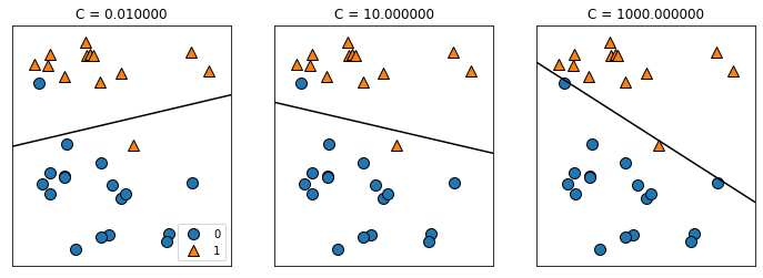
C = 0.01(규제가 강함): 비교적 수평에 가까운 결정 경계를 가지며 잘못 분류된 데이터 포인트는 2개이다.
C = 10.0: C = 0.01의 결정 경계 기울기만 달라짐
C = 1000(규제가 약함): 잘못 분류된 데이터 포인트는 1개 이며 클래스의 전체적인 배치를 파악하지 못하였기 떄문에 과대적합되었다고 볼 수 있다.

  
from sklearn.datasets import load_breast_cancer
cancer = load_breast_cancer()
# C = 1인 경우 --> 과소 적합(train set score과 test set score이 비슷)
X_train, X_test, y_train, y_test = train_test_split(cancer.data, cancer.target, stratify = cancer.target, random_state = 42)
logreg = LogisticRegression(max_iter = 5000).fit(X_train, y_train)
print("Training set score: {:.3f}".format(logreg.score(X_train, y_train)))
print("Test set score: {:.3f}".format(logreg.score(X_test, y_test)))

"""
Training set score: 0.958
Test set score: 0.958
"""

logreg100 = LogisticRegression(C = 100, max_iter = 5000).fit(X_train, y_train)
print("Training set score: {:.3f}".format(logreg100.score(X_train, y_train)))
print("Test set score: {:.3f}".format(logreg100.score(X_test, y_test)))

"""
Training set score: 0.984
Test set score: 0.965
"""

logreg001 = LogisticRegression(C = 0.01, max_iter = 5000).fit(X_train, y_train)
print("Training set score: {:.3f}".format(logreg001.score(X_train, y_train)))
print("Test set score: {:.3f}".format(logreg001.score(X_test, y_test)))

"""
Training set score: 0.953
Test set score: 0.951
"""

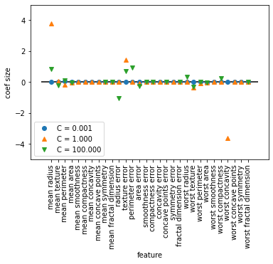
plt.plot(logreg100.coef_.T, '^',label = "C = 100")
plt.plot(logreg.coef_.T, 'o',label = "C = 1")
plt.plot(logreg.coef_.T, ' v', label = "C = 0.001")
plt.xticks(range(cancer.data.shape[1]), cancer.feature_names, rotation = 90)
xlims = plt.xlim()
plt.hlines(0, xlims[0], xlims[1])
plt.xlim(xlims)
plt.ylim(-5, 5)
plt.xlabel("feature")
plt.ylabel("coef size")
plt.legend()
plt.show()

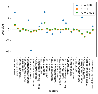
규제가 커지면 계수가 0에 가까워진다.
C = 100, C = 1 인 경우는 음수이다.
C = 0.001 인 경우는 양수이다.

즉, 계수가 클래스와 특성의 연관성을 알 수 있다.

ex) 계수와 클래스의 연관성

“texture error” : 양수 → 악성과 관련이 있음
“mean perimeter” : 계수의 부호가 변화함 → 양성 or 음성의 신호 모두가 될 수 있음

  
# L1 규제를 사용
for C, marker in zip([0.001, 1, 100],['o','^','v']):
  lr_l1 = LogisticRegression(solver = 'liblinear', C = C, penalty = 'l1', max_iter = 1000).fit(X_train, y_train)
  print("Training Accuracy of Logistic Regression with C = {:.3f}: {:.2f}".format(C, lr_l1.score(X_train, y_train)))
  print("Test Accuracy of Logistic Regression with C = {:.3f}: {:.2f}".format(C, lr_l1.score(X_test, y_test)))
  plt.plot(lr_l1.coef_.T, marker, label = "C = {:.3f}".format(C))

plt.xticks(range(cancer.data.shape[1]), cancer.feature_names, rotation = 90)
xlims = plt.xlim()
plt.hlines(0, xlims[0], xlims[1])
plt.xlabel("feature")
plt.ylabel("coef size")

plt.ylim(-5,5)
plt.legend(loc = 3)

"""
Training Accuracy of Logistic Regression with C = 0.001: 0.91
Test Accuracy of Logistic Regression with C = 0.001: 0.92
Training Accuracy of Logistic Regression with C = 1.000: 0.96
Test Accuracy of Logistic Regression with C = 1.000: 0.96
Training Accuracy of Logistic Regression with C = 100.000: 0.99
Test Accuracy of Logistic Regression with C = 100.000: 0.98
"""

다중 클래스 분류용 선형 모델

(로지스틱 회귀를 제외하고) 많은 선형 모델은 태생적으로 이진 분류만 지원

일대다(one-vs.-rest): 각 클래스를 다른 모든 클래스와 구분하도록 이진 분류 모델을 학습 → 클래스의 수만큼 이진 분류 모델이 만들어 모든 이진 분류기가 작동하여 가장 높은 점수를 내는 분류기의 클래스를 예측값으로 선택

즉, $w[0] * x[0] + w[1] * x[1] + … + w[p] * x[p] + b$의 값이 높은 클래스가 해당 데이터의 클래스 레이블로 할당한다.

  
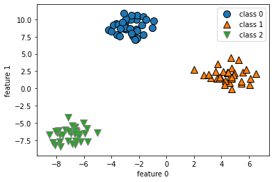
# dataset : 2차원
from sklearn.datasets import make_blobs

X, y = make_blobs(random_state = 42)
mglearn.discrete_scatter(X[:, 0], X[:, 1], y)
plt.xlabel("feature 0")
plt.ylabel("feature 1")
plt.legend(["class 0", "class 1","class 2"])
plt.show()

  
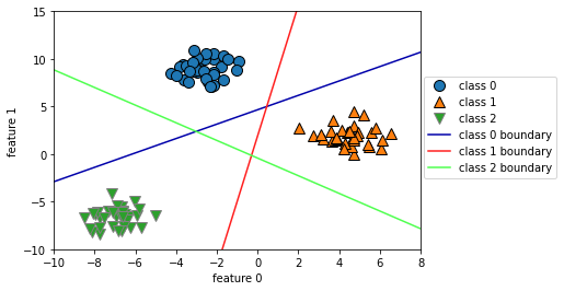
linear_svm = LinearSVC().fit(X, y)
print("size of coefficient array: ", linear_svm.coef_.shape)
print("size of intercept array: ", linear_svm.intercept_.shape)

"""
size of coefficient array:  (3, 2)
size of intercept array:  (3,)
"""

mglearn.discrete_scatter(X[:,0], X[:,1], y)
line = np.linspace(-15, 15)
for coef, intercept, color in zip(linear_svm.coef_, linear_svm.intercept_,mglearn.cm3.colors):
  plt.plot(line, -(line * coef[0] + intercept) / coef[1], c = color)
plt.ylim(-10,15)
plt.xlim(-10,8)
plt.xlabel("feature 0")
plt.ylabel("feature 1")
plt.legend(['class 0','class 1','class 2','class 0 boundary','class 1 boundary','class 2 boundary'], loc = (1.01, 0.3))
plt.show()

  
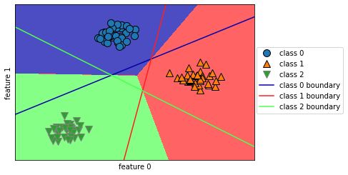
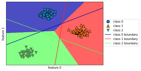
mglearn.plots.plot_2d_classification(linear_svm, X, fill = True, alpha = .7)
mglearn.discrete_scatter(X[:,0], X[:,1], y)
line = np.linspace(-15, 15)
for coef, intercept, color in zip(linear_svm.coef_, linear_svm.intercept_, mglearn.cm3.colors):
  plt.plot(line, -(line * coef[0] + intercept) / coef[1], c = color)
plt.legend(['class 0','class 1','class 2','class 0 boundary','class 1 boundary','class 2 boundary'],loc = (1.01, 0.3))
plt.xlabel("feature 0")
plt.ylabel("feature 1")
plt.show()

선형 모델	매개변수
회귀 모델	alpha
LinearsSVC	C
LogisticRegression	C

alpha가 커지면 모델이 단순해짐지고 C는 작아지면 모델이 단순해진다.

규제	특징
L1	중요한 특성이 많지 않을 때 사용 & 모델 해석이 중요한 요소일 때 사용
L2	기본적으로 많이 사용

그 중 L1은 해당 모델에 중요한 특성이 무엇이고 그 효과가 어느 정도인지 설명하기가 쉽다.

선형 모델의 장점

학습 속도가 빠르고 예측도 빠름.
매우 큰 데이터셋과 희소한 데이터셋에서도 잘 작동 (if. 대용량 데이터셋 → solver = ‘sag’ 옵션 or SGDClassifier, SGDPegressor 사용)
회귀와 분류에서 본 공식을 사용해 예측이 어떻게 만들어지는지 쉽게 이해할 수 있음 샘플에 비해 특성이 많을 때 잘 작동 → 매우 큰 데이터셋에 사용

선형 모델의 단점

계수의 값들이 왜 그런지 명확하지 않을 때가 있음. (데이터셋의 특성들이 서로 깊게 연관되어 있을 때 발생 → 계수 분석이 어려움)
저차원 데이터셋에는 성능이 좋지 않음

SGDClassifier & SGDRegressor

  
# SGDClassifier 모델로 훈련
from sklearn.linear_model import SGDClassifier
 
sgd_c = SGDClassifier(alpha = 0.01, learning_rate = 'adaptive', eta0 = 0.1, random_state = 42, n_jobs = -1)
sgd_c.fit(X, y)

mglearn.plots.plot_2d_classification(sgd_c, X, fill = True, alpha = .7)
mglearn.discrete_scatter(X[:,0], X[:, 1], y)
line = np.linspace(-15, 15)
for coef, intercept, color in zip(sgd_c.coef_, sgd_c.intercept_, mglearn.cm3.colors):
  plt.plot(line, -(line * coef[0] + intercept) / coef[1], c = color)
plt.legend(['class 0', 'class 1','class 2','class 0 boundary','class 1 boundary','class 2 boundary'], loc = (1.01, 0.3))
plt.xlabel("feature 0")
plt.ylabel("feature 1")
plt.show()

  
# SGDRegressor 모델로 훈련
from sklearn.linear_model import SGDRegressor

X, y = mglearn.datasets.load_extended_boston()
X_train, X_test, y_train, y_test = train_test_split(X,y, random_state = 0)

sgd_r = SGDRegressor(learning_rate = 'adaptive', eta0 = 0.1, random_state = 42)
sgd_r.fit(X_train, y_train)

print("Training set score: {:.2f}".format(sgd_r.score(X_train, y_train)))
print("Test set score: {:.2f}".format(sgd_r.score(X_test, y_test)))

"""
Training set score: 0.91
Test set score: 0.77
"""

Book, introduction-to-machine-Learning-with-python

ml python scikit-learn supervised-learning

This post is licensed under CC BY 4.0 by the author.

2.3 지도 학습 알고리즘

2.3.3 선형 모델

Trending Tags