[파이썬 라이브러리를 활용한 머신러닝] 비지도학습 및 데이터 전처리(1)

비지도 학습(unsuperivsed learning 이란?

• 알고 있는 출력값이나 정보 없이 학습 알고리즘을 자르쳐야 하는 모든 종류의 머신러닝
• 입력 데이터만으로 데이터에서 지식을 추출해야함

3.1 비지도 학습의 종류

---

비지도 변환(unsupervised transformation): 새롭게 표현하여 사람이나 다른 머신러닝 알고리즘에 원래 데이터보다 쉽게 해석할 수 있도록 만드는 알고리즘

• 차원 축소(dimensionality reduction): 특성이 많은 고차원 데이터를 특성의 술르 줄이면서 꼭 필요한 특징을 포함한 데이터로 표현하는 방법
  • 시각화를 위해 데이터셋을 2차원으로 변경하는 경우
• 데이터를 구성하는 단위나 성분 찾기
  • 많은 텍스트 문서에서 주제를 추출하는 것

군집(clustering) : 데이터를 비슷한 것끼리 그룹으로 묶는 방법

• 업로드한 사진을 분류할 때 같은 사람이 찍힌 사진을 같은 그룹으로 묶는 것

3.2 비지도 학습의 도전 과제

---

Goal: 알고리즘이 뭔가 유용한 것을 학습했는지 평가하는 것

보통 레이블이 없는 데이터에 적용하기 때문에 무엇이 올바른 출력인지 모르는 경우가 존재해 직접 확인하는 것이 유일한 방법일 떄가 많음

• 탐색적 분석 단계에서 많이 사용함

비지도 학습은 지도 학습의 전처리 단계에서도 사용

• 새롭게 표현된 데이터를 이용해 지도 학습의 정확도가 높아지기도 하며 메모리와 시간도 절약할 수 있음

스케일 조정은 비지도 방식으로 수행되는 전처리 기법이다.

pip install mglearn
pip install --upgrade joblib==1.1.0

import sklearn
import numpy as np
import matplotlib.pyplot as plt
import pandas as pd
import mglearn
import warnings
warnings.filterwarnings("ignore")

3.3 데이터 전처리와 스케일 조정

---

데이터의 특성 값을 조정 : 신경망이나 SVM 같은 데이터의 스케일에 민감하게 반응하는 알고리즘을 사용하는 경우

# 데이터셋의 스케일을 조정하거나 전처리하는 방법
mglearn.plots.plot_scaling()

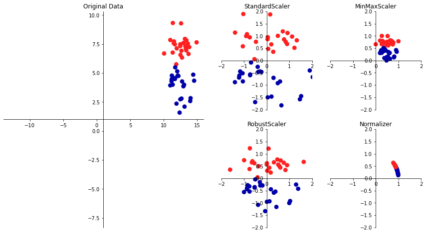
3.3.1 여러 가지 전처리 방법

• StandardScaler은 각 특성의 평균을 0, 분산을 1로 변경하여 모든 특성이 같은 크기를 가지게 하는 방법으로 특성의 최솟값과 최대값 크기를 제한하지 않는다.
• RobustScaler은 같은 스케일을 갖게 된다는 통계적 측면에서 StandardScaler과 비슷하지만 평균과 분산 대신 중간 값(median)과 사분위 값(quartile)을 사용하며 전체 데이터와 아주 동떨어진 데이터 포인트(이상치) 영향을 주지 않는다.

이상치(outlier): 보통 관측된 데이터의 범위에서 많이 벗어난 데이터

• MinMaxScaler은 정확하게 0과 1 사이에 위치하며 2차원 데이터셋인 경우, 모든 데이터가 x축의 0과 1, y축의 0과 1사이의 사각 영역에 존재한다.
• Normalizer는 특성 벡터의 유클리드안 길이가 1이 되도록 데이터 포인트를 조정되며 지름이 1인 원에 데이터 포인트를 투영 즉, 각 데이터 포인트가 다른 비율로 스케일이 조정된다. 또한, 특성 벡터의 길이는 상관없고 데이터의 방향(또는 각도)만이 중요하다.

3.3.2 데이터 변환 적용하기

스케일을 조정하는 전처리 메서드들은 보통 지도 학습 알고리즘을 적용하기 전에 적용한다.

from sklearn.datasets import load_breast_cancer
from sklearn.model_selection import train_test_split
cancer = load_breast_cancer()

X_train, X_test, y_train, y_test = train_test_split(cancer.data, cancer.target, random_state = 1)

print(X_train.shape)
print(X_test.shape)

"""
(426, 30)
(143, 30)
"""

from sklearn.preprocessing import MinMaxScaler

# 전처리
scaler = MinMaxScaler()
scaler.fit(X_train)

# 데이터 변환(스케일이 조정된 데이터 저장)
X_train_scaled = scaler.transform(X_train)
# 스케일이 조정된 후 데이터셋의 속성을 출력
print("변횐된 후 크기:", X_train_scaled.shape)
print("스케일 조정 전 특성별 최소값:\n", X_train.min(axis = 0))
print("스케일 조정 전 특성별 최대값:\n", X_train.max(axis = 0))
print("스케일 조정 후 특성별 최소값:\n", X_train_scaled.min(axis = 0))
print("스케일 조정 후 특성별 최대값:\n", X_train_scaled.max(axis = 0))

"""
변횐된 후 크기: (426, 30)
스케일 조정 전 특성별 최소값:
 [6.981e+00 9.710e+00 4.379e+01 1.435e+02 5.263e-02 1.938e-02 0.000e+00
 0.000e+00 1.060e-01 5.024e-02 1.153e-01 3.602e-01 7.570e-01 6.802e+00
 1.713e-03 2.252e-03 0.000e+00 0.000e+00 9.539e-03 8.948e-04 7.930e+00
 1.202e+01 5.041e+01 1.852e+02 7.117e-02 2.729e-02 0.000e+00 0.000e+00
 1.566e-01 5.521e-02]
스케일 조정 전 특성별 최대값:
 [2.811e+01 3.928e+01 1.885e+02 2.501e+03 1.634e-01 2.867e-01 4.268e-01
 2.012e-01 3.040e-01 9.575e-02 2.873e+00 4.885e+00 2.198e+01 5.422e+02
 3.113e-02 1.354e-01 3.960e-01 5.279e-02 6.146e-02 2.984e-02 3.604e+01
 4.954e+01 2.512e+02 4.254e+03 2.226e-01 9.379e-01 1.170e+00 2.910e-01
 5.774e-01 1.486e-01]
스케일 조정 후 특성별 최소값:
 [0. 0. 0. 0. 0. 0. 0. 0. 0. 0. 0. 0. 0. 0. 0. 0. 0. 0. 0. 0. 0. 0. 0. 0.
 0. 0. 0. 0. 0. 0.]
스케일 조정 후 특성별 최대값:
 [1. 1. 1. 1. 1. 1. 1. 1. 1. 1. 1. 1. 1. 1. 1. 1. 1. 1. 1. 1. 1. 1. 1. 1.
 1. 1. 1. 1. 1. 1.]
"""

# 테스트 데이터 변환
X_test_scaled = scaler.transform(X_test)
# 스케일이 조정된 후 테스트 데이터의 속성을 출력
print("스케일 조정 후 특성별 최소값:\n", X_test_scaled.min(axis = 0))
print("스케일 조정 후 특성별 최대값:\n", X_test_scaled.max(axis = 0))

"""
스케일 조정 후 특성별 최소값:
 [ 0.0336031   0.0226581   0.03144219  0.01141039  0.14128374  0.04406704
  0.          0.          0.1540404  -0.00615249 -0.00137796  0.00594501
  0.00430665  0.00079567  0.03919502  0.0112206   0.          0.
 -0.03191387  0.00664013  0.02660975  0.05810235  0.02031974  0.00943767
  0.1094235   0.02637792  0.          0.         -0.00023764 -0.00182032]
스케일 조정 후 특성별 최대값:
 [0.9578778  0.81501522 0.95577362 0.89353128 0.81132075 1.21958701
  0.87956888 0.9333996  0.93232323 1.0371347  0.42669616 0.49765736
  0.44117231 0.28371044 0.48703131 0.73863671 0.76717172 0.62928585
  1.33685792 0.39057253 0.89612238 0.79317697 0.84859804 0.74488793
  0.9154725  1.13188961 1.07008547 0.92371134 1.20532319 1.63068851]
"""

• 전처리는 훈련 데이터로만 fit()하고, 테스트 데이터에는 transform()만 적용해야 한다.
  • 테스트 데이터는 훈련 기준으로 변환되므로, 0~1 범위를 벗어날 수도 있음.
• 테스트에 fit()을 하면 데이터 누수가 발생해 모델 성능이 부정확하게 평가된다.

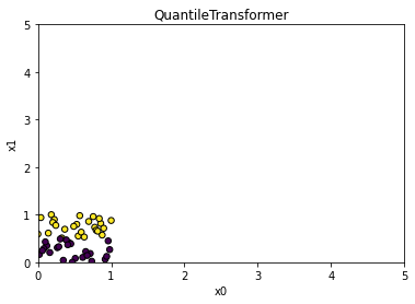
3.3.3 QuantileTransformer와 PowerTransformer

QuantileTransformer : 1,000개의 분위를 사용하여 데이터를 균등하게 분포시킴(scikit-learn 0.19.0 에 추가)

• 이상치에 민감하지 않음
• 전체 데이터를 0과 1사이로 압축

import matplotlib.pyplot as plt
import numpy as np
from sklearn.datasets import make_blobs
from sklearn.preprocessing import QuantileTransformer, StandardScaler, PowerTransformer

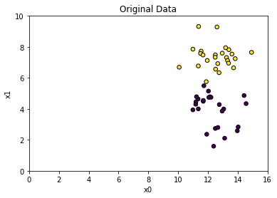
X, y = make_blobs(n_samples = 50, centers = 2, random_state = 4, cluster_std = 1)
X += 3

plt.scatter(X[:, 0], X[:, 1], c = y, s = 30, edgecolors = 'black')
plt.xlim(0, 16)
plt.xlabel('x0')
plt.ylim(0, 10)
plt.ylabel('x1')
plt.title("Original Data")
plt.show()

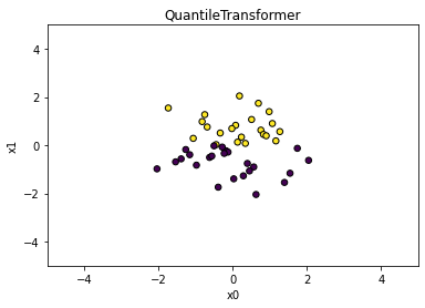
scaler = QuantileTransformer(n_quantiles = 50)
X_trans = scaler.fit_transform(X)

plt.scatter(X_trans[:,0], X_trans[:, 1], c = y, s = 30, edgecolors = 'black')
plt.xlim(0, 5)
plt.xlabel('x0')
plt.ylim(0, 5)
plt.ylabel('x1')
plt.title(type(scaler).__name__)
plt.show()

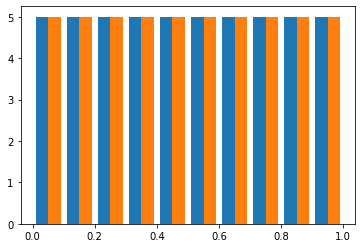
# 균등 분포
plt.hist(X_trans)
plt.show()

print(scaler.quantiles_.shape)

# (50, 2)

x = np.array([[0],[5],[8],[9],[10]])
print(np.percentile(x[:, 0], [0,25, 50, 75, 100]))

# [ 0.  5.  8.  9. 10.]

x_trans = QuantileTransformer(n_quantiles = 5).fit_transform(x)
print(np.percentile(x_trans[:, 0], [0, 25, 50, 75, 100]))

# [0.   0.25 0.5  0.75 1.  ]

# output_distribution : normal 균등 분포 --> 정규 분포
scaler = QuantileTransformer(output_distribution = 'normal', n_quantiles = 50)
X_trans = scaler.fit_transform(X)

plt.scatter(X_trans[:, 0], X_trans[:, 1], c = y, s = 30, edgecolors = 'black')
plt.xlim(-5, 5)
plt.xlabel('x0')
plt.ylim(-5, 5)
plt.ylabel('x1')
plt.title(type(scaler).__name__)
plt.show()

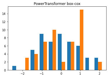
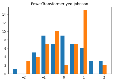
PowerTransformer : 데이터의 특성별롤 정규분포 형태에 가깝도록 변환(scikit-learn 0.20.0 버전에 추가)

• method 매개변수 : yeo-johnson, box-cox
• 기본값 : yeo-johnson

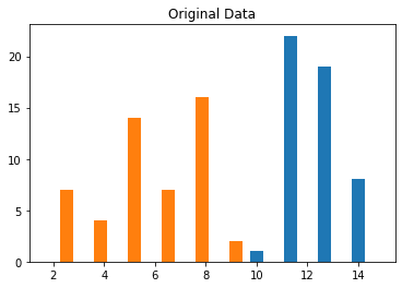
plt.hist(X)
plt.title('Original Data')
plt.show()

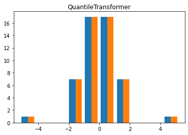
X_trans = QuantileTransformer(output_distribution = 'normal', n_quantiles = 50).fit_transform(X)
plt.hist(X_trans)
plt.title('QuantileTransformer')
plt.show()

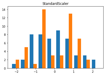
X_trans = StandardScaler().fit_transform(X)
plt.hist(X_trans)
plt.title('StandardScaler')
plt.show()

X_trans = PowerTransformer(method = 'box-cox').fit_transform(X)
plt.hist(X_trans)
plt.title('PowerTransformer box-cox')
plt.show()

X_trans = PowerTransformer(method = 'yeo-johnson').fit_transform(X)
plt.hist(X_trans)
plt.title('PowerTransformer yeo-johnson')
plt.show()

3.3.4 훈련 데이터와 테스트 데이터의 스케일을 같은 방법으로 조정하기

지도 학습 모델에서 테스트 세트를 사용하려면 훈련 세트와 테스트 세트에 같은 변환을 적용해야한다.

from sklearn.datasets import make_blobs
# 인위적인 데이터셋 생성
X, _ = make_blobs(n_samples = 50, centers = 5, random_state = 4, cluster_std = 2)
# 훈련 세트와 테스트 세트로 나누기
X_train, X_test = train_test_split(X, random_state = 5, test_size = .1)
# 훈련 세트와 테스트 세트의 산점도 그리기
fig, axes = plt.subplots(1, 3, figsize = (13, 4))
axes[0].scatter(X_train[:, 0], X_train[:, 1], c = mglearn.cm2.colors[0], label = "Training set", s = 60)
axes[0].scatter(X_test[:, 0], X_test[:, 1], marker = '^', c = mglearn.cm2.colors[1], label = "Test set", s = 60)
axes[0].legend(loc = 'upper left')
axes[0].set_title("Original data")

# MinMaxScaler를 사용해 스케일을 조정
scaler = MinMaxScaler()
scaler.fit(X_train)
X_train_scaled = scaler.transform(X_train)
X_test_scaled = scaler.transform(X_test)

# 스케일이 조정된 데이터의 산점도를 그림
axes[1].scatter(X_train_scaled[:, 0], X_train_scaled[:, 1], c=mglearn.cm2(0),label="Training set", s=60)
axes[1].scatter(X_test_scaled[:, 0], X_test_scaled[:, 1], marker='^', c=mglearn.cm2(1), label="Test set", s=60)
axes[1].set_title("Scaled Data")

# 테스트 세트의 스케일을 따로 조정
# 테스트 세트의 최솟값은 0, 최댓값은 1
# 예제를 위한 것, 잘못 사용된 예제
test_scaler = MinMaxScaler()
test_scaler.fit(X_test)
X_test_scaled_badly = test_scaler.transform(X_test)

# 잘못 조정된 데이터의 산점도를 그림
axes[2].scatter(X_train_scaled[:, 0], X_train_scaled[:, 1], c=mglearn.cm2(0), label="training set", s=60)
axes[2].scatter(X_test_scaled_badly[:, 0], X_test_scaled_badly[:, 1], marker='^', c=mglearn.cm2(1), label="test set", s=60)
axes[2].set_title("Improperly Scaled Data")

for ax in axes:
    ax.set_xlabel("Feature 0")
    ax.set_ylabel("Feature 1")
fig.tight_layout()

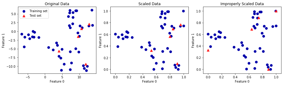
• 첫 번째 그래프 : 2차원 원본 그래프
• 두 번째 그래프 : MinMaxScaler로 스케일을 조정한 그래프
  • 훈련 세트와 테스트 세트에 동일한 transform 메서드를 적용
  • 축의 눈금만 바뀌고 첫 번째 그래프와 동일
  • 모든 특성은 0과 1 사이에 놓여 있음
  • 테스트 데이터(삼각형)의 최솟값과 최댓값은 0과 1이 아님
• 세 번쨰 그래프 : 스케일을 서로 다른 방식을 조정
  • 훈련 세트와 테스트 세트의 최솟값과 최댓값이 모두 0과 1임
  • 원본 데이터와 매우 다름
  • 배열이 매우 뒤죽박죽되었음

# 단축 메서트와 효율적인 방법
from sklearn.preprocessing import StandardScaler
scaler = StandardScaler()
# 메소드 체이닝(chaining)을 사용하여 fit과 transform을 연달아 호출
X_scaled = scaler.fit(X_train).transform(X_train)
# 위와 동일하지만 더 효율적
X_scaled_d = scaler.fit_transform(X_train) # 모든 모델에서 효율적 X

3.3.5 지도 학습에서 데이터 전처리 효과

SVC을 이용하여 원래 데이터와 MinMaxScaler, StandScaler 결과를 비교하여 전처리 효과를 확인할 수 있다.

from sklearn.svm import SVC
X_train, X_test, y_train, y_test = train_test_split(cancer.data, cancer.target, random_state = 0)

svm = SVC(gamma = 'auto')
svm.fit(X_train, y_train)
print("Test set accuracy: {:.2f}".format(svm.score(X_test, y_test)))

# Test set accuracy: 0.63

# 0-1 사이로 스케일 조정
scaler = MinMaxScaler()
scaler.fit(X_train)
X_train_scaled = scaler.transform(X_train)
X_test_scaled = scaler.transform(X_test)

# 조정된 데이터로 SVM 학습
svm.fit(X_train_scaled, y_train)

# 스케일 조정된 테스트 세트의 정확도
print("Scaled Test set accuracy: {:.2f}".format(svm.score(X_test_scaled, y_test)))

# Scaled Test set accuracy: 0.95

# 평균 0, 분산 1을 갖도록 스케일 조정
from sklearn.preprocessing import StandardScaler
scaler = StandardScaler()
scaler.fit(X_train)
X_train_scaled = scaler.transform(X_train)
X_test_scaled = scaler.transform(X_test)

# 조정된 데이터로 SVM 학습
svm.fit(X_train_scaled, y_train)
# 스케일 조정된 테스트 세트의 정확도
print("SVM test accuracy: {:.2f}".format(svm.score(X_test_scaled, y_test)))

# SVM test accuracy: 0.97